For starters you won’t be able to do the earthcache
observations if the Little Miami river level is too high. Check
here for the river level.
Little Miami River Level
The river was at 5.5 feet when I made my observations. If the
water is a few feet higher and the GZ will be under water and you
won’t be able to take your measurements. You should be
standing in the middle of the rock “beach” on the shore
of the Little Miami River. Note for paperless cachers – this
might be one cache worth printing out to help with the field
work.
There is no need to bushwhack. There is a well-defined trail in
Avoca park that starts at N 39° 08.343 W 084° 20.478 Parking is
near there too. This is why I selected this spot – easy
access!
Where you are standing is a point bar of a river meander or a
sharp bend in the river. For more info on how meanders are formed
and their features visit GC36NKM. Both this
“beach” of rock and the deeply eroded bank on the
opposite side were formed by the two processes that shape river
geography, erosion and sedimentation. What we are going to do at
this spot is to quantify the driving force of erosion: the velocity
of the water!
When the river is at flood stage, very fast moving water scrubs
the point bar you are standing on. Note the uniformity of the rocks
at this spot. They are all scrubbed white – no algae, no dirt
on the rocks. They are almost entirely composed of rocks that have
sides eroded round by the erosive power of the water. They also
almost have a distinctive shape: mostly flat. It is the fast
flowing flood water that basically “sorts” these rocks,
leaving these here on the bank while washing others downstream or
left deeper in the channel bed. The flow also scrubs off the dirt
and smaller particles like sand off this area. The only smaller
rocks you see might be lodged under some of the larger ones.
Henning Filip Hjulstrom was a Swedish geographer who started
quantifying the processes that form features like this point bar.
Below is a notional version of the diagram he and his students
later developed to quantify erosion and deposition of river
materials.
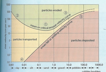
This is a graph that shows the relationship between the size of
sediment and the velocity required to erode (lift it), transport it
and deposit it. The critical erosion curve shows the MINIMUM
velocity required to lift a particle of a certain size. The mean
fall or “settling” deposition curve shows the MAXIMUM
velocity at which a river can be flowing before a particle of a
certain size is deposited. The zone in-between is the zone of
transport. Note the velocities for transport are lower than that
for erosion, because it takes much more energy to lift sediment and
start its motion than to maintain it in transport. Note that the
graph is logarithmic, not linear. On this scale you can see that
from 1mm to 100mm the “transportation” velocity, or the
velocity that a particle will be moved, is linear relative to
particle size. But below 1mm the relation between particle diameter
and velocity is not as well correlated.
This curve shape is due to the fact that there are two different
regimes covered by the graph. For particle sizes where friction is
the dominating force preventing erosion (1-100mm) the graph is
linear. But for cohesive material like clay and silt, the erosion
velocity increases with decreasing grain size, as the cohesive
forces (electrostatic) are relatively more important. Note the
consistency of the material under/between the rocks – thick
clay and mud.
Estimating River Velocity
We are going to use the graph below to estimate the water
velocity scrubbing this point bar. From where you are standing try
to find the smallest rock that is on the top layer. We’ll
assume the water current was fast enough to wash away anything
smaller. The motion of rocks along the bottom of a river is called
“bed load”. The curve lists “diameter” and
assumes spherically shaped objects (sand perhaps), but the rocks at
the GZ are more ellipsoid in shape – like the diagram below.
So we’ll come up with an equivalent diameter.

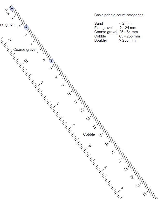
For you paperless earthcachers, I’ll try to describe the
dimensioning. Almost all the rocks you’ll see around you are
relatively flat on one side with an oval shaped face. Dimension
“C” is the thinnest dimension between the 2 flat faces.
If you look at the oval face of the rock “A” is the
longest dimension and “B” is the direction
perpendicular to “A”. (If you printed out the cache
listing there’s a scale at the bottom.). Measure B and C. (If
you don’t have a scale and didn’t print this out you
could take a photo next to your GPS to scale it on the computer
screen.)
We’ll assume the rocks tend to line themselves up with the
water flow such that water flows along the “A”
dimension. Then the “B” and “C” dimensions
set the ellipse shaped cross section of the rock. The chart lists
velocities based on diameter so we’ll estimate the equivalent
diameter based on cross sectional area. The circular cross
sectional area of a sphere is where D is the diameter =
Π[pi]x(D)(D)/4 for our ellipse it is Π[pi] x(B)(C). So
measuring the dimensions B and C for the rock - use the following
to calculate the equivalent diameter for the chart.
√ (4)(B)(C)
[Again for you paperless cachers that’s square root of the
product 4xBxC.]
With this “effective” diameter you can go into the
detailed Hjulstrom curve and pick off the velocity of the water
that it would take to move it. Remember it’s a log/log
curve.
Now we’ll add one last scientific detail to our
calculation. We’ll also assume the coefficient of drag of the
flat rock (an ellipsoid) is one half that of a sphere (per
http://www.alepuniv.edu.sy/ev/uploaded_files/elibrary/files/file_667_828122.pdf)
so the water velocity to move an ellipsoid rock is twice what you
got from the curve. From that, you know that the velocity of the
water there is a little less, but not much less or smaller rocks
would be present.

To see a neat video of bed load transport - see the YouTube
video below.
http://www.youtube.com/watch?v=o3llzwvv1zc
To log this earthcache email me the answers to the following:
(Show your math!)
1) What are the dimensions of your rock (B and C)?
2) What is it’s equivalent diameter?
3) Which of the two curves on the Hjulstrom diagram do you use
to determine the velocity
required to start the motion of your rock that is at rest (this
is the curve to use to answer #4)?
4) What water velocity would it take to move your rock? (You can
convert to mile per hour using 1 centimeter/second = 0.022 369 362
921 mile/hour (mph))
5) The curve provided is for a water depth of 1 meter. Check out
the river bank. The wall of dirt marks the “bank full”
height of the river. When the river rises above this the water
spills out onto the vegetated flood plain above. So is the curve
applicable here?
6) Based on the charts how is your rock classified? (pebble,
cobble, etc) Use the sizing on the diagram not the ruler.
7) Optional: post a picture of yourself and your rock to
commemorate your visit!
Scale: